Recently some colleagues and I were finalizing a paper on the generalizability of scores coming from an experimental design. One of the ideas that shortly crossed our minds was whether such a generalizability study could be approached with a Bayesian flavour. At that time we decided to put that idea in the fridge but it kept coming back to my mind. This post can be seen as the result of that brooding and I’m very curious to hear your ideas on this. Does it make sense to approach it in this way or not?
I will start with a very rough sketch of the purpose of Generalizability Theory. This sketch is undeniably inadequate, but I provide readers who are interested in this subject with the necessary references. Then I introduce a fictitious example, a case study: Maare’s Vegan Burgers. First, I approach the data belonging to this case in a frequentist manner, and then I apply a Bayesian sauce to it. I am curious to see whether you will like this post and look forward to your reactions.
The following packages are needed throughout the post:
Generalizability theory: an inadequate intro
Before we delve into the example and the analyses, let us first introduce very very roughly the idea behind Generalizability Theory. Most of what I’ll write is based on the article of Bloch and Norman (2012). If you’re looking for a great introduction into this topic, the article of Bloch and Norman (2012) (the title “Generalizability Theory for the Perplexed” says it all) is the place to start.
To put it short, generalizability can be seen as an extension of the concept of reliability in classical test theory (CTT). Reliability of scores are typically determined by an index that indicates the ratio of the variance in the signal to the variance in the noise. For instance, if we are giving 10 year olds a math test of 10 questions, a reliability coefficient will express the amount of variance in scores that is due to real differences between our 10 year olds rather than variance due to measurement error (coming from using 10 questions).
In generalizability theory a more flexible framework is developed allowing to take care of multiple sources of measurement error. Let us imagine the following situation. With some friends you are playing at a soccer field and you start to bet who can kick a ball the furthest on the pitch. One problem that you have is that you don’t have a good measurement tool to measure the distance. You come up with the following procedure. All 11 of the friends kick a ball at their turn. Each time a ball is kicked 4 random friends start to measure the distance in steps and you take the average of these 4 friends’ amount of steps as a measure of distance to decide who has won that cool drink. In this situation there are multiple sources of possible error that enter the measurement system. First, it is not unimaginable that each person will differ in how large the steps are that she or he takes. Moreover, even if you would let all the measurements be done by the same 4 friends, on each occasion (for each kick) there will be some random variance entering the measurement system because we cannot expect that people are 100% consistent in the length of the steps they take. So these are already two sources of measurement error that can be identified. This is where Generalizability theory kicks in. It offers a framework to think about the measurement design and express the uncertainty in scores coming from multiple sources of measurement error build in the design. Typically a well designed Generalizability study will result in a generalizability coefficient that can be interpreted as the relative amount of variance in scores that can be ascribed to true variance. So a generalizability coefficient of 0.70 means that 70% of the differences in scores can be seen as true score variance while the other 30% of the differences comes from the measurement error induced by the measurement design which may incorporate different sources of measurement error.
I hope this gives a very rough idea about the aim of Generalizability theory and the associated analyses. These analyses typically rely on some procedure to estimate different variances in the frequentist way. Let us introduce a case study for which we will have some data and do the analyses.
The case: Maare burgers
Maare has just started a sustainable vegan takeaway restaurant. She wants to put a burger on the menu that will also please real meat-eaters. After extensive market research, she has found five different producers of vegan burgers. Now, of course, she has the question: which burger to choose as the basis for the Maare Burger? A brief discussion with her partner tells her that the best thing to do is to set up a proper survey in which the public is asked to judge the burgers. After some brainstorming, they came up with a few factors that could influence the scores that the burgers receive:
- The customers (tastes differ);
- The chef who prepares the burgers (3 different chefs will alternate in the kitchen later, so she wants to reflect this in her study).
Time for a study, they thought. Maare placed an appeal on the social media for participants and found 60 volunteers. They are invited on a sunny Sunday for lunch and will eat and judge the burgers. Each chef will prepare 20 Maare Burgers using the products of that day, four per brand of vegan burger. Participants will give a rating on 10 for the burger they ate, resulting in a dataset with 60 ratings.
The study design looks like this: 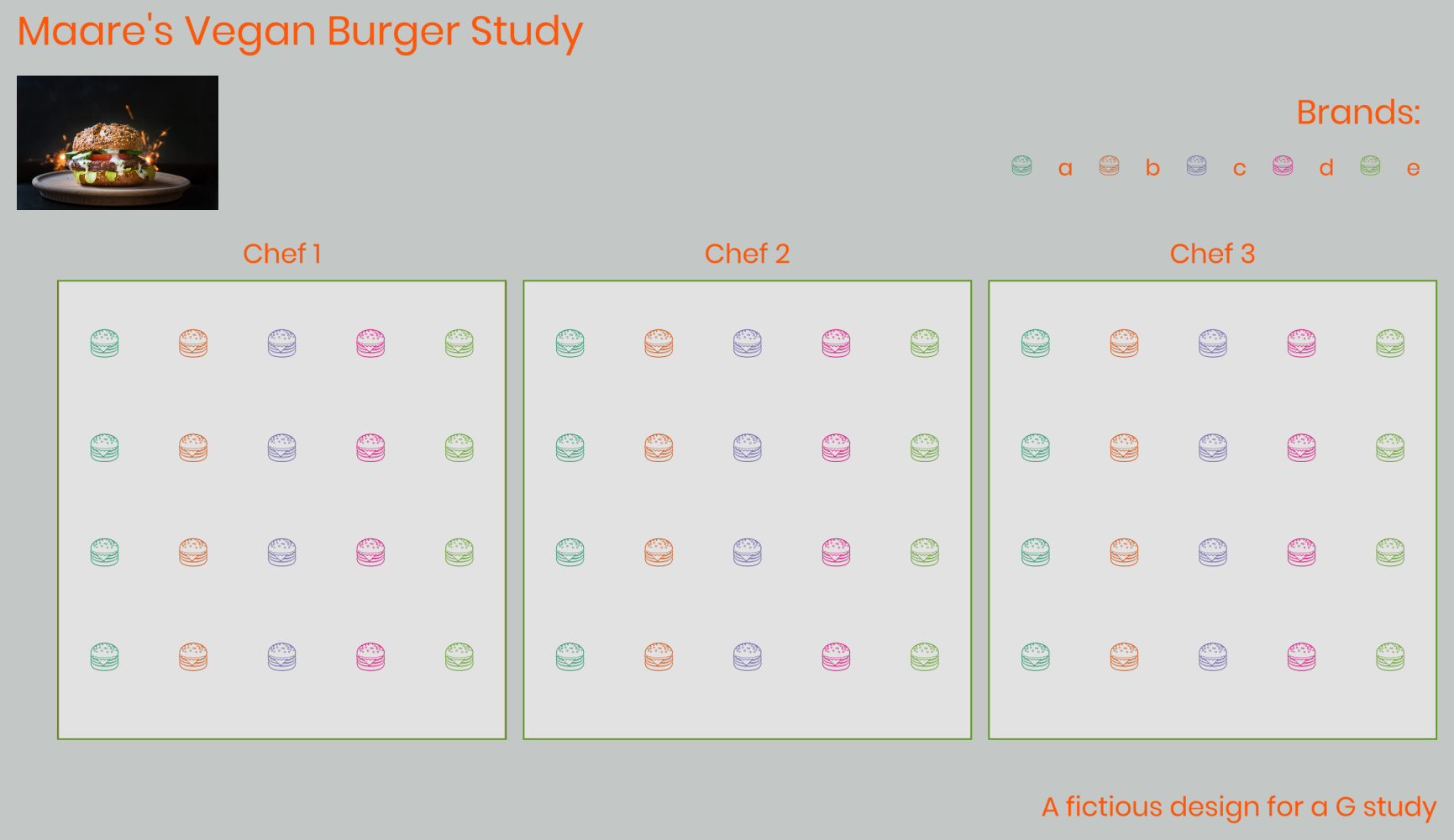
When discussing their design with a friend of them who studies psychometrics, they received a very critical question:
“Do you think you will be able to generalize your findings to other situations when you have other customers or other chefs preparing the burgers?”
This friend suggested to conduct a “Generalizability study” based on the data they gathered on that sunny Sunday.
The fictitious data that I crafted for this post is called Burgers. More specifically the subset of scores in that dataset for day_id == 1. So let’s load the data and create a subset called Day1.
A quick plot of the data gives some idea of the variance in scores and the differences between the five brands.
Show code
Day1 %>%
  ggplot(aes(x = Brands, y = dv, color = factor(chef_id))) +
  geom_jitter(alpha = 0.6, width = 0.2) +
  scale_y_continuous(name = "Score") +
  labs(color = "Chef") +
  theme(legend.position = "top")
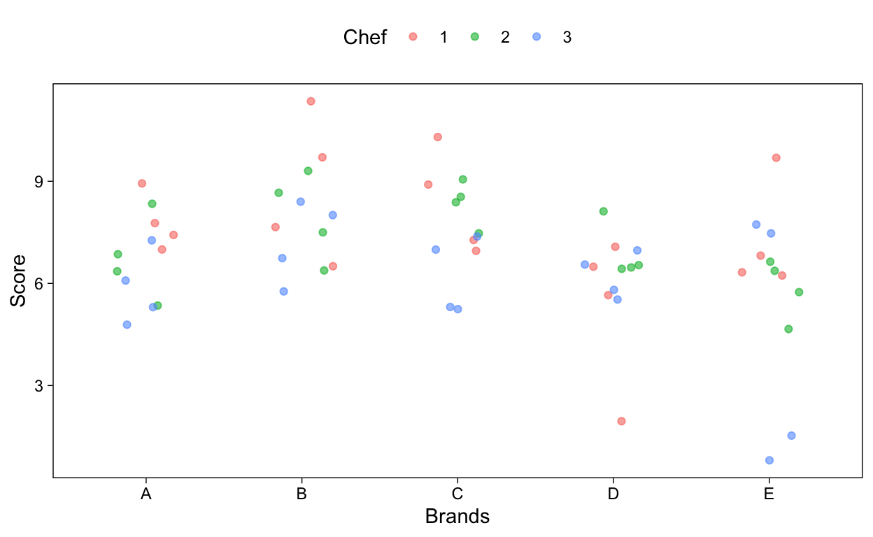
Figure 1: Jitter plot of scores assigned to the Maare burgers per brand
Generalizability the frequentist way
With the design of Maare’s small study in mind we can frame the generalizability question as follows:
If we have ratings of 20 burgers how much of the differences in ratings between these burgers can be ascribed to actual differences between the burgers and how much is due to the chef or the customers?
A frequentist way to do the analyses to estimate the variances needed to calculate the generalizability is relying on a mixed effects analyses in lme4. In the dataset we have the scores stored in the variable dv. The variable chef_id identifies the chef who made the burger and the variable burger_id identifies the nth burger made by that chef.
Show code
 Groups    Name        Variance
 burger_id (Intercept) 0.2894
 chef_id   (Intercept) 0.2925
 Residual              2.8578
With these variance estimates we can start calculating the generalizability coefficient by using the following formula:
\[ G = \frac{var(\text{burgers})}{var(\text{burgers})+\frac{var(\text{chefs})}{\text{n chefs}}+\frac{var(\text{error})}{\text{(n chefs * n burgers)}}} \]
In R this is an easy task:
Show code
G_lmer <- 0.2894 /
  (0.2894 + (0.2925 / 3) + (2.8578 / (3*20)))

G_lmer
[1] 0.666007So, the generalizability is lower than 0.7 what sometimes is used as a reference to say that the generalizability is sufficient (e.g. Bloch and Norman (2012)).
A typical step now would be to perform a decision study where we simulate new scenarios and investigate the impact on the generalizability. In the next piece of code I simulate that the number of burgers per chef would vary from 2 to 50 (see the variable nBurgers created). The generalizability coefficient is calculated for each of these scenarios and both are plotted:
Show code
nBurgers <- seq(from = 2, to = 50)

Dstudy_lmer <- 0.2894 /
  (0.2894 + (0.2925 / 3) + (2.8578 / (3*nBurgers)))

tibble(nBurgers,Dstudy_lmer) %>%
  ggplot(aes(x=nBurgers,y=Dstudy_lmer)) +
  geom_line() +
  geom_hline(yintercept = 0.7, color = "#D95F02", lty =2) +
  scale_y_continuous(name = "Generalizability",
                     breaks = c(.4 , .5, .6, .7, .8),
                     limits = c(0.3,0.85))+
  scale_x_continuous(limits = c(0,50))
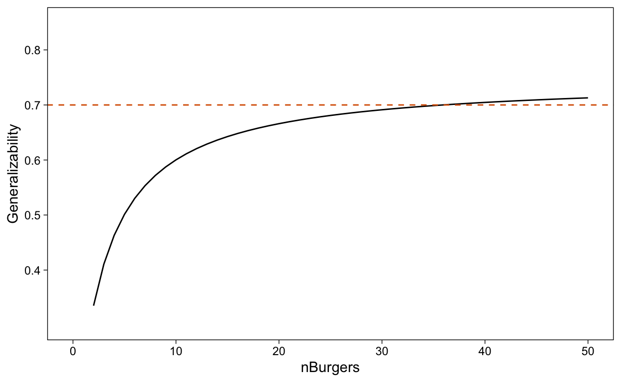
Figure 2: How the generalizability depends on the number of burgers in the study
From this plot we can learn that Maare has to ask each chef to prepare around 35 burgers that can be tasted and rated to result in a sufficient generalizability coefficient.
Generalizability the Bayesian (brms) way
In what we have done until now is giving Maare a point-estimate of the generalizability of scores for burgers coming from her market study. We relied on variance estimates without factoring in the uncertainty of these estimates. The Bayesian framework, however, gives us every opportunity to do so. After all, using a Bayesian analysis, we can estimate a posterior distribution for the various variance estimates that includes the uncertainty regarding our estimates.
To do this, I like to fall back on brms as a package in R where we can do this very easily since the formula notation of brms is parallel to how it is also implemented in lme4 (see Bürkner 2017, 2018).
Before we start with the actual estimation of the model, it is wise to consider our priors for the different parameters in the model. Through brms we get uninformative priors by default. However, we may have some more prior knowledge here.
For example, we might already assume in advance that the scores on a scale of 10 are on average rather positive and thus land around 7 points on average. For this, we can rely on Maare’s domain knowledge.She selected the best brands for which she had already read very good reviews. Since there is still uncertainty about the average score we can expect, we can translate this uncertainty into the prior by using, for example, the normal distribution with a mean of 7 and standard deviation of 1.5 points. In addition, we also have an idea about the differences between the chefs and the differences between the citizens: these will be there anyway and may well increase in sd’s. Therefore, we use a t-distribution with a mean of 0.2, an sd of 1 and a 1 degree of freedom (such that the tails are also reasonably thick and thus also capture the chance that the differences between chefs or between citizens are large). We do the same for the final error variance (sigma), but with a mean of 1 to take into account that this error variance is clearly greater than the other two sources of variance. In R we can visualise these priors as follows to give a better idea of our expectations.
Show code
library(metRology)
x <- seq(0,10,by=0.1)


sd_burger_and_chef <- dt.scaled(x, 1, 0.2, 0.5)
sigma     <- dt.scaled(x, 1,   1, 0.5)
intercept <- dnorm(x, 7, 1.5)

Priors <-
  data_frame(x, sd_burger_and_chef, sigma, intercept) %>%
  pivot_longer(c(sd_burger_and_chef, sigma, intercept),
               names_to="Prior") %>%
  mutate(
   model_part = ifelse(Prior == "intercept", "intercept", "variances")
  ) %>%
  ggplot(aes(x = x, y = value, color = Prior)) +
  geom_line() +
  scale_x_continuous(name = "") +
  facet_wrap(.~model_part)

Priors
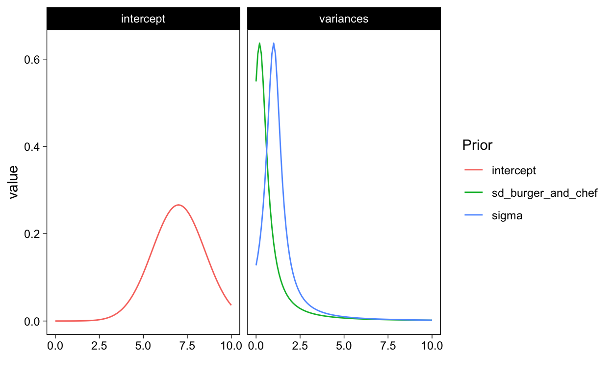
Figure 3: Prior probability distributions for the parameters in the model
Now that we have decided on the priors we are ready to define the model in brms and estimate the model:
Show code
prior_brms_model <- c(
  set_prior("normal(7,1.5)", class = "Intercept"),
  set_prior("student_t(1,0.2,0.5)", class = "sd", group = "burger_id"),
  set_prior("student_t(1,0.2,0.5)", class = "sd", group = "chef_id"),
  set_prior("student_t(1,1,0.5)", class = "sigma")
  )

brms_model <-
  brm(dv ~ 1 +
        (1|burger_id) +
        (1|chef_id),
      warmup = 1500,
      iter = 3000,
      data = Day1,
      prior = prior_brms_model,
      control = list(adapt_delta = 0.99),
      backend = "cmdstanr"
      )

saveRDS(brms_model, file = "fitted_models/brms_model.RDS")
Show code
brms_model <- readRDS(file = "fitted_models/brms_model.RDS")
Based on our analyses we can visualize the uncertainty on the variance parameters as follows:
Show code
posterior_samples(brms_model) %>%
   mutate(
    var_chef = sd_chef_id__Intercept^2,
    var_burger = sd_burger_id__Intercept^2,
    var_sigma = sigma^2
    ) %>%
  select(var_burger, var_chef, var_sigma) %>%
  pivot_longer(everything()) %>%
  ggplot(aes(x = value, y = 0)) +
   stat_halfeye(.width = c(.50,.89,.95),
                     normalize = "panels") +
   scale_y_continuous(NULL, breaks = NULL) +
   xlab("marginal posterior") +
   facet_wrap(~name, scales = "free", ncol = 1)
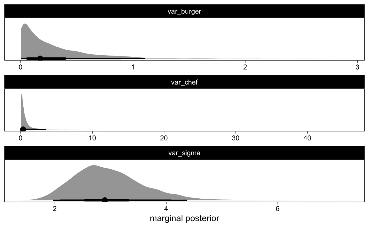
Figure 4: Posterior distribution for the variance parameters in the model
These plots demonstrate the large amount of uncertainty we still have concerning the variance estimates for both the variance between chefs and the variance between the burgers. This does not come as a surprise given the rather small number of chefs and burgers per chef that we have in our data.
Of course the main goal of our analysis is to estimate the generalizability. One way to plot the posterior distribution of this coefficient is as follows (notice how easy it is to calculate with our posterior samples…):
Show code
posterior_samples(brms_model) %>%
  mutate(
    var_chef = sd_chef_id__Intercept^2,
    var_burger = sd_burger_id__Intercept^2,
    var_sigma = sigma^2
    ) %>%
  mutate(
    Generalizability = var_burger /
              (var_burger + (var_chef / 3) + (var_sigma^2 / (3*20)))  # calculate the Generalizability
  ) %>%
  select(Generalizability) %>%
  pivot_longer(everything()) %>%
  ggplot(aes(x = value, y = 0, fill = stat(x > 0.7))) +
   stat_halfeye(.width = c(.50,.89,.95),
                     normalize = "panels") +
   scale_y_continuous(NULL, breaks = NULL) +
   xlab("marginal posterior") +
   facet_wrap(~name, scales = "free") +
  labs(fill = "Meets the 0.7?") +
  theme(legend.position = "top")
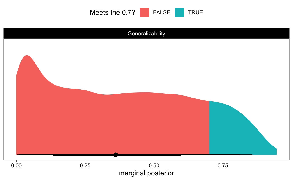
Figure 5: Posterior distribution for the Generalizability coefficient of differences between burgers
It goes beyond discussion that we are not that certain about how generalizable the differences between burgers are, given the design of Maare’s study. The majority of credible values for the generalizability coefficient are situated in the region lower than 0.7. We can also calculate the probability of getting a Generalizability coefficient highter than 0.7 making use of the information in our posterior.
Show code
posterior_samples(brms_model) %>%
  mutate(
    var_chef = sd_chef_id__Intercept^2,
    var_burger = sd_burger_id__Intercept^2,
    var_sigma = sigma^2
    ) %>%
  mutate(
    Generalizability = var_burger /
              (var_burger + (var_chef / 3) + (var_sigma^2 / (3*20)))  # calculate the Generalizability
  ) %>%
  mutate(
    G_sufficient = ifelse(Generalizability > 0.70, "Yes", "No")
  ) %>%
  group_by(G_sufficient) %>%
  summarize(
    n_draws = (n()/6000)
  ) %>%
  DT::datatable(
    colnames = c("Is G larger than 0.7?", "Probability"),
    rownames = F
  ) %>% formatPercentage('n_draws', 2)
So there is 15% probability that the generalizability of the ratings are sufficient. This uncertainty around the generalizability coefficient is also apparent when we translate these findings into a D-study. The following plot contains the generalizability coefficient as a function of the number of burgers, including a 50%, 80% and 95% credible interval. These large intervals indicate how uncertain we are about the impact of the number of burgers on the generalizability coefficient!
Show code
Posterior_estimates <-
  posterior_samples(
  brms_model
  ) %>%
  mutate(
    var_chef = sd_chef_id__Intercept^2,
    var_burger = sd_burger_id__Intercept^2,
    var_sigma = sigma^2
    ) %>%
  mutate(
    draw_id = seq(1, 6000)
  ) %>%
  select(
    draw_id,
    var_chef,
    var_burger,
    var_sigma
  )


crossing(draw_id = seq(1,6000), nBurgers = seq(from = 2, to = 50)) %>%
  left_join(Posterior_estimates, by = "draw_id") %>%
  mutate(
    G_coeff = var_burger /
              (var_burger + (var_chef / 3) + (var_sigma / (3*nBurgers)))  # calculate the Generalizability
  ) %>%
  ggplot(aes(x = nBurgers, y = G_coeff)) +
  stat_lineribbon(aes(y = G_coeff), color = "#D95F02") +
  scale_fill_brewer(palette = "Greys") +
  ylab("Generalizability") +
  xlab("number of burgers")
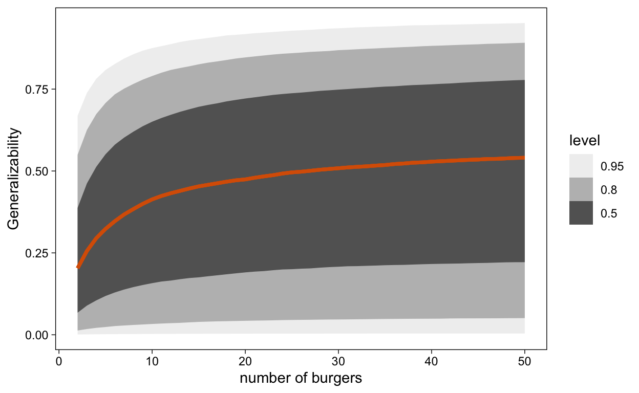
Figure 6: D-study with the incorporated uncertainty as contained in the posterior printed as CI’s
Another way to visualize this uncertainty is by drawing a random sample of 100 possible generalizability coefficients and draw a function for each of these draws and the relation with the number of burgers.
Show code
Posterior_estimates <-
  posterior_samples(
  brms_model,
  subset = (sample(seq(1,6000), 100)) # sample 100 parameter estimates out of the 6000
  ) %>%
  mutate(
    var_chef = sd_chef_id__Intercept^2,
    var_burger = sd_burger_id__Intercept^2,
    var_sigma = sigma^2
    ) %>%
  mutate(
    draw_id = seq(1, 100)
  ) %>%
  select(
    draw_id,
    var_chef,
    var_burger,
    var_sigma
  )


Plot <-
  crossing(draw_id = seq(1,100), nBurgers = seq(from = 2, to = 50)) %>%
  left_join(Posterior_estimates, by = "draw_id") %>%
  mutate(
    G_coeff = var_burger /
              (var_burger + (var_chef / 3) + (var_sigma / (3*nBurgers)))  # calculate the Generalizability
  ) %>%
  ggplot(aes(x = nBurgers, y = G_coeff)) +
  geom_line(aes(y = G_coeff, group = draw_id), color = "#D95F02") +
  ylab("Generalizability") +
  xlab("number of burgers") +
  transition_states(draw_id, 0, 1) +
  shadow_mark(future = TRUE, color = "gray50", alpha = 1/20)

animate(Plot, nframes = 50, fps = 2.5, width = 864, height = 576, res = 128, dev = "png", type = "cairo")
Figure 7: D-study based on 100 posterior draws (each line is a credible link between number of burgers and the generalizability coefficient)
Wrap-up
Maare may have a very rough idea about how much she can trust the scores coming from her experiment. For us, I hope this fictitious example illustrated the idea to perform Generalizability theory analyses making use of a Bayesian approach. I am very curious to hear your thoughts on this. Does this make sense? What can be improved? Any further suggestions? Let me know!
Appendix: the code to create the dataset
With this code you can create the dataset used in this post. It even results in a larger dataset with multiple days rather than one day. So you can start playing around with the more complex data if you wish!
Show code
library(tidyverse)
library(tibble)

nChefs <- 3
nBrands <- 5
nOccasions <- 4
nBurgers_Chef_Brands <- 4

nBurgers_Chef_Occasion <- nBrands * nBurgers_Chef_Brands
nBurger_Occasion <- nChefs * nBurgers_Chef_Occasion
nBurger_Total <- nBurger_Occasion * nOccasions

OccLabel <- c("Day 1", "Day 2", "Day 3", "Day 4")
names(OccLabel) <- c(1:4)

ChefLabel <- c("Chef 1", "Chef 2", "Chef 3")
names(ChefLabel) <- c(1:3)

# Create random effects Judges

n_judges <- 60
judge_sd <- 1.49

set.seed(2020)

Judges <- tibble::tibble(
  judge_id = seq(1:n_judges),
  judge_i  = rnorm(n_judges, 0, judge_sd),
 )

ggplot(Judges, aes(judge_i)) +
  geom_density()

# Create random effects Day

n_days <- 4
days_sd <- 0.11

set.seed(2020)

Days <- tibble::tibble(
  day_id = seq(1:n_days),
  day_i  = rnorm(n_days, 0, days_sd)
  )

# Create random effects Chef

n_chefs  <- 3
chefs_sd <- 0.89

set.seed(2020)

Chefs <- tibble::tibble(
  chef_id = seq(1:n_chefs),
  chef_i  = rnorm(n_chefs, 0, chefs_sd)
  )

Burgers <- tibble::tibble(
  burger_id = seq(1:nBurgers_Chef_Occasion)
  )

# Create 240 trials (of which we will only use Day1 data)

trials <- crossing(
  day_id = Days$day_id,         # get days IDs from the simulated data table
  chef_id = Chefs$chef_id,      # get chefs IDs from the simulated data table
  burger_id = Burgers$burger_id
  ) %>%
  left_join(Days, by = "day_id") %>%  # includes the intercept for each day
  left_join(Chefs, by = "chef_id")    # includes the intercept for eachchef

# Assign judges to trials

set.seed(1)
Order_day1 <- sample(seq(1:60),60)
set.seed(2)
Order_day2 <- sample(seq(1:60),60)
set.seed(3)
Order_day3 <- sample(seq(1:60),60)
set.seed(4)
Order_day4 <- sample(seq(1:60),60)

Judges_rating <-
  rbind(Judges[Order_day1,],
      Judges[Order_day2, ],
      Judges[Order_day3, ],
      Judges[Order_day4, ])

Brands <- rep(LETTERS[seq(1:5)], 48)

trials <- trials %>%
  cbind(Judges_rating) %>%
  cbind(Brands) %>%
  mutate(
    Brand_A = ifelse(Brands == "A", 1, 0),
    Brand_B = ifelse(Brands == "B", 1, 0),
    Brand_C = ifelse(Brands == "C", 1, 0),
    Brand_D = ifelse(Brands == "D", 1, 0),
    Brand_E = ifelse(Brands == "E", 1, 0)
  )


# set variables to use in calculations below

grand_i          <-  7.00
brand_B_eff      <-  0.80
brand_C_eff      <-  0.46
brand_D_eff      <- -0.95
brand_E_eff      <- -1.10
error_sd         <-  0.12

# Bring it all together and create the dataframe with column dv containing the simulated scores

dat <- trials %>%
  mutate(
    # calculate error term (normally distributed residual with SD set above)
    err = rnorm(nrow(.), 0, error_sd),
    # calculate DV from intercepts, effects, and error
    dv = grand_i + judge_i + chef_i + day_i + err +
      (brand_B_eff * Brand_B) +
      (brand_C_eff * Brand_C) +
      (brand_D_eff * Brand_D) +
      (brand_E_eff * Brand_E)
  )