If you get confronted with colleagues that apply Bayesian analyses you’ll notice that they use a specific vocabulary: “prior distribution”, “posterior distribution”, “Highest Probability Density Intervals”, “MCMC”,… But what’s the meaning of these words? And how to make sense out of all these Bayesian mishmash? After some reading around (and learning of course) I started to get a first understanding of some key concepts. And now I want to share my insights with you.
In this post I’ll try to explain the basics and explain 4 key concepts. But before that, a short sidestep on the goal of stats (because sometimes we seem to forget).
Stats? Why?
To put it simple: stats help us to model reality in numbers and assist us in getting better insight in the world. Let’s say we have a major concern on the rise of vampires in Europe 1. Rumours are getting spread saying that the almost 20% of the Europeans is actually a vampire, but nobody really has a good idea on the number of vampires. The major question then is: how many vampires are out there? This is a statistical question that can be approached by a pretty simple model: the proportion of vampires among the whole population of Europeans. This model only contains one unknown value: the actual proportion of vampires. This unknown value is what we often call a parameter. We can calculate the exact proportion in the exceptional case that we can test every single one of the whole European population. But that’s utopia. In research most of the time we make use of samples (we test a random chosen number of European citizens) and we do not calculate the exact parameter value. We estimate the parameter value. Statistics helps us to estimate parameter values. But it does even more. Good statistics also quantifies the (un)certainty on our parameter estimate(s)! If we apply this to our question concerning the proportion of vampires, we want statistics to help us quantify how certain we are about different proportions of vampires as the true proportion in the population.
This brings us to our two first concepts from Bayesian analysis: priors and posteriors.
Priors and posteriors
Bayesian statistics calls the quantification of uncertainty on parameter estimates priors and posteriors. So both concepts refer to some kind of probability.
Lets start with the prior.
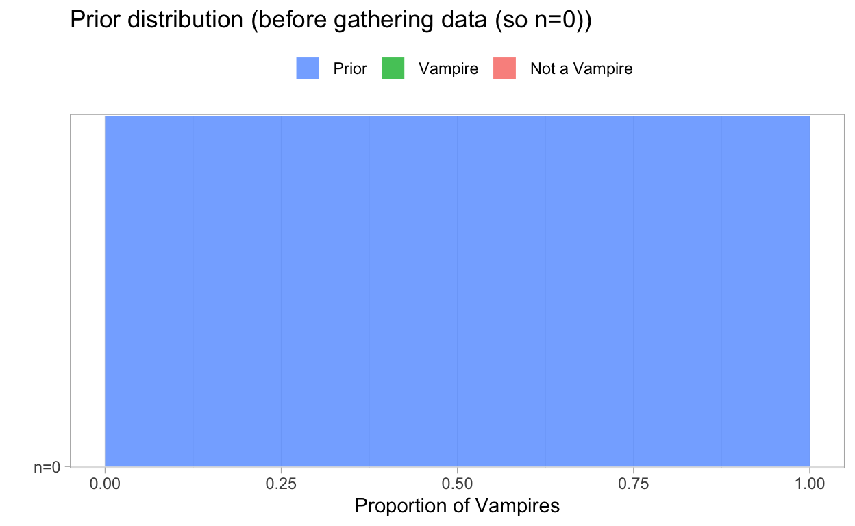
A prior is a quantification of (un)certainty on parameter estimates that we have before we consider the information in the data that we gather.
Back to our example of vampires. A prior can quantify our prior knowledge on the probability that any possible proportion of vampires is the true proportion in Europe. Now, imagine that we do not have any clue before we start our research then each proportion has the same probability. The following plot shows our prior! Note that we have no data yet. So this graph visualizes our prior knowledge about the proportion of vampires.
Of course, in research we gather data. In our example we’re lucky that we have prof. dr. Van Helsing 2. He’s a famous professor who developed the ultimate Vampire Test that determines whether a person is a vampire or not. As a successful professor he was able to get research funding from the European Commission. In his step of the research he had the silly idea to gather data in a sample of n=1: he tested one random European citizen. And the result was that this random person is not a vampire. Now, given his data we can update our knowledge on our parameter. We now know that it is impossible that 100% of the Europeans are vampires. So we adapt our pior probability to what is called a posterior probability! The next plot shows what happens. The red area in the graph is our posterior distribution, demonstrating that we no longer assign any probability that the proportion of vampires is 100% and that the probabilities increase as the proportion of vampires decreases.
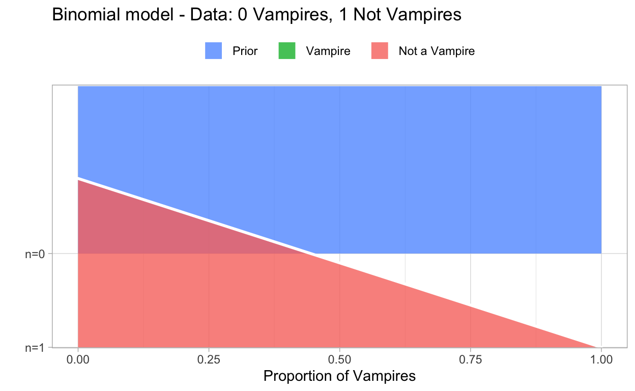
A posterior is a quantification of (un)certainty on parameter estimates that we have taking into account the information in the data that we gather.
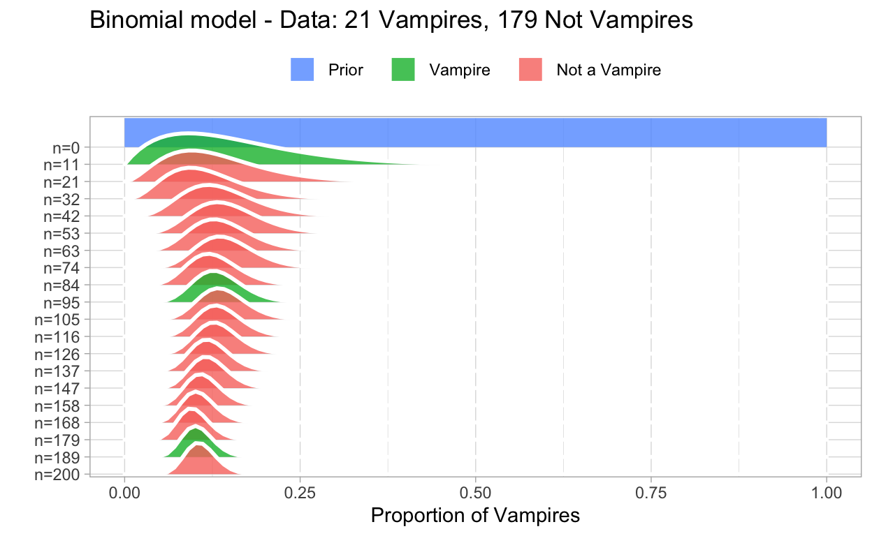
In work package 2 prof. dr. Van Helsing was able to draw a random sample of 200 Europeans and he applied his test. This resulted in data containing 21 vampires and 179 normal persons. This data can be used to update our knowledge on our parameter. The result is visualized in the next plot where the curve (and area) plotted at line “n=200” is actually the posterior probability distribution for our parameter.
We can actually zoom in to our posterior distribution that looks like this:
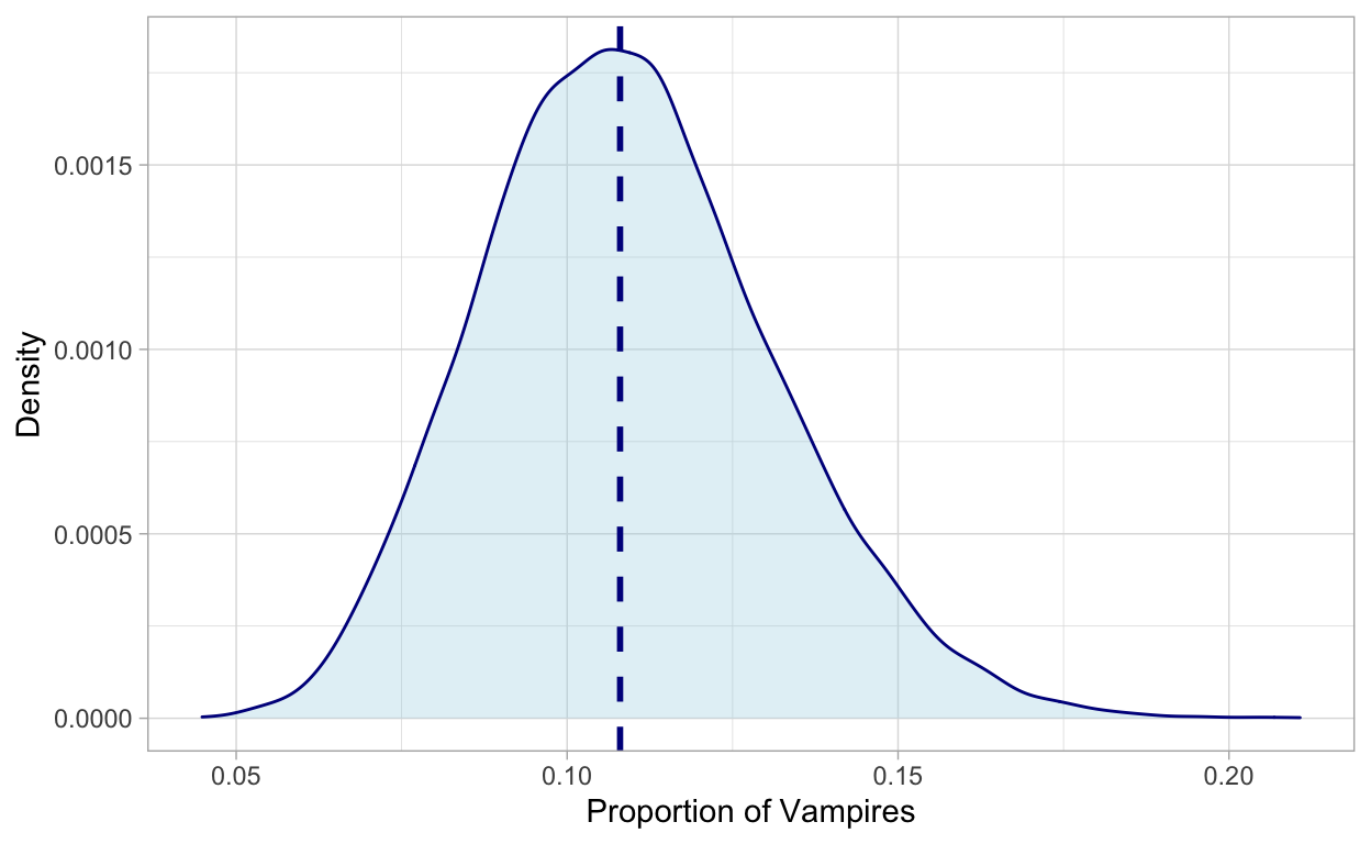
The dashed line indicates the median of our posterior distribution which can be seen as the most probable proportion of vampires in Europe (being 0.107 or 10.7%) given our sample. But other proportions are plausible as well. To help us with making inferences to the population based on our posterior probability distribution, we can make use of a HPDI!
HPDI
In comes our third term: the Highest Probability Density Interval (HPDI).
An HPDI is an interval between two parameter values (limits) that contain a predefined number of most plausible parameter values.
This definition may sound a bit abstract, but if we apply it to our example it will hopefully become more clear. First, we have to define how large an interval we wish. For example, we could be interested in the 90% most plausible parameter estimates. So, we construct a 90% HPDI. Let’s apply this to our example:
Concerning the proportion of vampires our posterior learns us that the 90% most plausible proportions of vampires are situated between 7.5% and 14.7%. Notice that the 20% vampires in Europe, the number being mentioned in some rumours, is not within this interval. As usual, do not always take rumours too seriously.
Still one concept to go: MCMC. But before we can do this we should dive into the Bayesian Theorem as until now we didn’t explain how we can update our priors to result in posteriors. The core of this proces is the Bayesian Theorem.
Bayesian Theorem
Bayesian analysis has received this name because at the heart of this type of analysis is the Bayesian Theorem that is used to update prior probabilities into posterior probabilities. The Bayesian Theorem is formally the following:
\[Pr(B|A) = \frac{Pr(A|B)*Pr(A)}{Pr(B)}\]
That looks complex and is typical probability theory stuff. In textbooks on Bayesian analyses this theorem is explained into detail. But, in my opinion for now it is more interesting to show you how this theorem is applied on priors and posteriors. In Bayesian analysis we are interested in the probability of parameter values given the data, something we earlier on labelled as the posterior (probability). If we apply the Bayesian theorem to this probability then we can write it down like this:
\[Pr(parameter|Data) = \frac{Pr(Data|parameter)*Pr(parameter)}{Pr(Data)}\]
This formula states how we can calculate the posterior. If we replace some terms by more meaningful terms it can become more clear what’s happening:
\[Posterior = \frac{Pr(Data|parameter)*Prior}{Pr(Data)}\]
How the other unknown terms are calculated \(Pr(Data|parameter)\) and \(Pr(Data)\) is something that can be learned in specific textbooks. More importantly I hope you get the idea! The only thing left to explain is how it works now. What does the estimation process look like? Time to introduce MCMC…
MCMC
The estimation process of Bayesian analyses can take many forms. The basic idea is that the formula from above is applied to each possible value of a paramater. In our vampire example this would imply that we do a calculation for each possible value between 0% vampires and 100% vampires so that each possible proportion gets an associated posterior probability. For a model like ours with only one parameter this is a job that may be handled easily by our modern computers 3. Of course, in real life research we apply more complex models. Imagine that you want to apply this to a regression model with 3 independent variables. The equation looks something like this:
\[Y_i = \beta_0 * Cons + \beta_1 * X_1 + \beta_2 * X_2 + \beta_3 * X_3 + \epsilon_i\]
This model contains 5 parameters to estimate! And even more importantly, a very very large number of combinations of parameter values for these parameters can be made. If we had to calculate the posterior probability for each and every possible combination we would have to wait for hours (or days, or weeks) before our computer throws back the results to us. This is where MCMC comes in the picture!
In the search for more efficient ways to apply Bayesian analyses, researchers have developed a smart sampling method: Markov Chain Monte Carlo (MCMC) sampling.
MCMC is a sampling method used in many scientific fields and also used in Bayesian statistical estimation. The sampling method is not random but uses an informed algorithm to sample the most informative samples of values of the parameter space.
The take-away message is that this MCMC sampling is a more efficient way to sample combinations of parameter values. In Bayesian analysis this sampling technique is applied and for each sample of parameter values the algorithm calculates the posterior distribution. By repeating this sampling a large number of times we get enough information to build a completer picture of the posterior distribution for all parameter values.
to end…
I hope you have some first impressions or ideas about the meaning of these key concepts in Bayesian analysis. Of course, it is way more complex than described in this blogpost. If you are triggered to learn more consider following sources (among the many out there).
Some url’s
https://rdrr.io/cran/brms/: info brms pakket
https://mjskay.github.io/tidybayes/index.html: info tidybayes pakket
https://www.rensvandeschoot.com/bayesian-analysis-informed-priors/: site van rens vandeschoot
http://www.sumsar.net/: site van Rasmus Bååth
Some great books
The book Statistical Rethinking from Richard McElreath (which also has associated youtube movies explaining each chapter!)
Another classical is Doing Bayesian Data Analysis (aka the doggy book) from John K. Kruschke.
If you have any suggestions, comments or questions concerning this blog or something related, please do not hesitate to contact me.
Ok. We can have serious doubts about whether this is the best example to demonstrate how we model reality↩︎
Prof.dr. Van Helsing first appeared in the novel “Dracula”. He’s the vampire hunter.↩︎
note that you still would have to decide how fine grained you want to do this (e.g. in steps of 1% each time resulting in 100 posterior probabilities or in steps of 0.0001% each time 1 000 000 posterior probabilities↩︎